ME 467 Project 1
Caleb Hottes, Charles Friley
Introduction
This project is focused on the simulation and analysis of a Furuta Pendulum using the mujoco and spatial math python libraries. It outlines the math needed to solve the analysis questions posed in the instructions document and uses the mujoco library to verify the analytical results and perform a simulation of an unrelated actuation. The methods and results are outlined in detail in this document, however the actual implementation of these calculations and obviously simulations was done in the attacked jupyter notebook files.
Position-Level Kinematics (Question 1)
Introduction
In this section we will resolve the position-level forward and inverse kinematics of the Furuta pendulum with the help of the coordinate systems as shown in the figure.
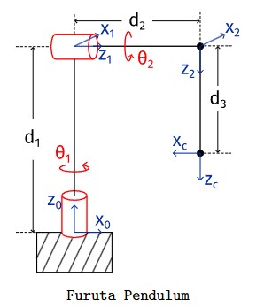
Parts a, b, and c of question 1 will be shown simultaneously and parts d and e will be shown separately after.
Methodology and Results
Parts A, B, and C
To start, we will first determine the position level kinematics of frame c and frame 2 in respect to frame 0 (${}^0T_c$ and ${}^0T_2$). To do this we first construct all the rotation and position matrixes from frame 0 to frame c by inspection.
The positions can be constructed by inspection.
$${}^0t_1 = \left[\begin{matrix}0\\0\\d_{1}\end{matrix}\right], {}^1t_2 = \left[\begin{matrix}0\\0\\d_{2}\end{matrix}\right], {}^2t_c = \left[\begin{matrix}0\\0\\d_{3}\end{matrix}\right]$$
The rotations are simple to construct.
From 0 to 1, we first rotate about $x$ by $\pi/2$, then we rotate about $y$ by $\theta_{1}$.
$$R_{x, \pi/2} R_{y, \theta_{1}} = {}^0R_1 = \left[\begin{matrix}\cos{\left(\theta_{1} \right)} & 0 & \sin{\left(\theta_{1} \right)}\\\sin{\left(\theta_{1} \right)} & 0 & - \cos{\left(\theta_{1} \right)}\\0 & 1 & 0\end{matrix}\right]$$
From 1 to 2, we first rotate about $x$ by $\pi/2$, then we rotate about $y$ by $\theta_{2}$.
$$R_{x, \pi/2} R_{y, \theta_{2}} = {}^1R_2 = \left[\begin{matrix}\cos{\left(\theta_{2} \right)} & 0 & \sin{\left(\theta_{2} \right)}\\\sin{\left(\theta_{2} \right)} & 0 & - \cos{\left(\theta_{2} \right)}\\0 & 1 & 0\end{matrix}\right]$$
From 2 to c, we just rotate about $z$ by $-\pi/2$.
$$R_{z, -\pi/2} = {}^2R_c = \left[\begin{matrix}0 & 1 & 0\\-1 & 0 & 0\\0 & 0 & 1\end{matrix}\right]$$
From these, the homogenous representation of the pose can be constructed.
$$ {}^0T_1 = \left[\begin{matrix}\cos{\left(\theta_{1} \right)} & 0 & \sin{\left(\theta_{1} \right)} & 0\\\sin{\left(\theta_{1} \right)} & 0 & - \cos{\left(\theta_{1} \right)} & 0\\0 & 1 & 0 & d_{1}\\0 & 0 & 0 & 1\end{matrix}\right]$$
$$ {}^1T_2 = \left[\begin{matrix}\cos{\left(\theta_{2} \right)} & 0 & \sin{\left(\theta_{2} \right)} & 0\\\sin{\left(\theta_{2} \right)} & 0 & - \cos{\left(\theta_{2} \right)} & 0\\0 & 1 & 0 & d_{2}\\0 & 0 & 0 & 1\end{matrix}\right]$$
$$ {}^2T_c = \left[\begin{matrix}0 & 1 & 0 & 0\\-1 & 0 & 0 & 0\\0 & 0 & 1 & d_{3}\\0 & 0 & 0 & 1\end{matrix}\right]$$
With these poses the desired pose can be constructed.
$$^{0}T_{c} = {}^{0}T_{1} \, {}^{1}T_{2} \, {}^{2}T_{c}$$
$$^{0}T_{2} = {}^{0}T_{1} \, {}^{1}T_{2} $$
Which results in:
$$^{0}T_{c} = \left[\begin{matrix}- \sin{\left(\theta_{1} \right)} & \cos{\left(\theta_{1} \right)} \cos{\left(\theta_{2} \right)} & \sin{\left(\theta_{2} \right)} \cos{\left(\theta_{1} \right)} & d_{2} \sin{\left(\theta_{1} \right)} + d_{3} \sin{\left(\theta_{2} \right)} \cos{\left(\theta_{1} \right)}\\\cos{\left(\theta_{1} \right)} & \sin{\left(\theta_{1} \right)} \cos{\left(\theta_{2} \right)} & \sin{\left(\theta_{1} \right)} \sin{\left(\theta_{2} \right)} & - d_{2} \cos{\left(\theta_{1} \right)} + d_{3} \sin{\left(\theta_{1} \right)} \sin{\left(\theta_{2} \right)}\\0 & \sin{\left(\theta_{2} \right)} & - \cos{\left(\theta_{2} \right)} & d_{1} - d_{3} \cos{\left(\theta_{2} \right)}\\0 & 0 & 0 & 1\end{matrix}\right]$$
$$ ^{0}T_{2} = \left[\begin{matrix}\cos{\left(\theta_{1} \right)} \cos{\left(\theta_{2} \right)} & \sin{\left(\theta_{1} \right)} & \sin{\left(\theta_{2} \right)} \cos{\left(\theta_{1} \right)} & d_{2} \sin{\left(\theta_{1} \right)}\\\sin{\left(\theta_{1} \right)} \cos{\left(\theta_{2} \right)} & - \cos{\left(\theta_{1} \right)} & \sin{\left(\theta_{1} \right)} \sin{\left(\theta_{2} \right)} & - d_{2} \cos{\left(\theta_{1} \right)}\\\sin{\left(\theta_{2} \right)} & 0 & - \cos{\left(\theta_{2} \right)} & d_{1}\\0 & 0 & 0 & 1\end{matrix}\right] $$
Plugging in the values of $\theta$ from part a of question 1, $\theta_1 = \pi/3$ and $\theta_2=-3\pi/7$ we find that:
$$ ^{0}T_{c} = \left[\begin{matrix}-0.5 & -0.193 & 0.844 & 1.075\\-0.866 & 0.111 & -0.487 & 0.303\\0.0 & -0.975 & -0.223 & 1.022\\0.0 & 0.0 & 0.0 & 1.0\end{matrix}\right] $$
$$ ^{0}T_{2} = \left[\begin{matrix}-0.193 & 0.5 & 0.844 & 0.4\\0.111 & 0.866 & -0.487 & 0.693\\-0.975 & 0.0 & -0.223 & 1.2\\0.0 & 0.0 & 0.0 & 1.0\end{matrix}\right] $$
The rotation matrix can be extracted:
$$ ^{0}R_{c} = \left[\begin{matrix}-0.5 & -0.193 & 0.844\\-0.866 & 0.111 & -0.487\\0.0 & -0.975 & -0.223\end{matrix}\right] $$
$$ ^{0}R_{2} = \left[\begin{matrix}-0.193 & 0.5 & 0.844\\0.111 & 0.866 & -0.487\\-0.975 & 0.0 & -0.223\end{matrix}\right] $$
Which can then be represented both as a unit quaternion and as a axis-angle. We used the r2q() function for the quaternion representation and tr2angvec() function for the axis angle representation, both from Spatial Math.
The quaternion representing $^{0}R_{c}$ is:
$$\ 0.3117 < -0.3909, 0.6771, -0.5400 > $$
The quaternion representing $^{0}R_{2}$ is: $$ 0.6022 < 0.2024, 0.7552, -0.1614 > $$
The axis angle representation of $^{0}R_{c}$ is:
$$ Angle: 2.508 \ rad \\ Axis: \left[\begin{matrix}-0.411 & 0.713 & -0.568\end{matrix}\right]$$
The axis angle representation of $^{0}R_{2}$ is: $$ Angle: 1.849 \ rad \\ Axis: \left[\begin{matrix}0.253 & 0.946 & -0.202\end{matrix}\right] $$
The rotation matrix can be recovered from the axis-angle representation by using rodrigues formula.
$ R = e^{\widehat{\omega} \theta} = \mathbf{I} + \sin(\theta) \widehat{\omega} + (1 - \cos(\theta)) \widehat{\omega}^2 $
Where:
- $\omega$ is the axis of rotation, a unit vector that defines the direction of rotation.
- $\theta$ is the scalar part of the axis-angle rotation, representing the rotation magnitude in radians.
- $\widehat{\omega}$ is the skew-symmetric matrix of $\omega$, used to compute the rotation matrix.
- $\mathbf{I}$ is the identity matrix.
Implementing this formula allowed us to recover the rotation matrix.
$$ ^{0}R_{c} = \left[\begin{matrix}-0.5 & -0.193 & 0.844\\-0.866 & 0.111 & -0.487\\0.0 & -0.975 & -0.223\end{matrix}\right] $$
$$ ^{0}R_{2} = \left[\begin{matrix}-0.193 & 0.5 & 0.844\\0.111 & 0.866 & -0.487\\-0.975 & 0.0 & -0.223\end{matrix}\right] $$
Part D
If camera is installed at the end-effector of the Furuta pendulum, what are the values of $ \theta_1 $ and $ \theta_2 $ if the $ z $-axis of the camera points in the direction $ k $, where
$$ k = -\frac{1}{2} x_0 + \frac{1}{2} y_0 - \frac{\sqrt{2}}{2} z_0. $$
In order to solve this question, we need to find the solutions for $\theta_1$ and $\theta_2$ in this equation:
$$ \begin{bmatrix} \ {}^0z_{c,1} \\ \ {}^0z_{c,2} \\ \ {}^0z_{c,3} \end{bmatrix} = \begin{bmatrix} k_1 \\ k_2 \\ k_3 \end{bmatrix} $$ Where $^0z_c$ is the $z$ part of $^{0}R_{c}$. Plugging in values: $$ \begin{bmatrix} \sin{\left(\theta_{2} \right)} \cos{\left(\theta_{1} \right)} \\ \sin{\left(\theta_{1} \right)} \sin{\left(\theta_{2} \right)} \\ - \cos{\left(\theta_{2} \right)} \end{bmatrix} = \begin{bmatrix} -0.5 \\ 0.5 \\ - \frac{\sqrt{2}}{2} \end{bmatrix} $$
We plugged these formulas into the solve() function in SymPy. This produced four potential solutions, which we then checked by plugging those $\theta$ values back into the forward kinematic equations to see if the resulting orientation matches that of the desired orientation. Only two of the four solution pairs were correct:
$$ \begin{align*} (\theta_1, \theta_2) &= (-0.785, 5.498),\\ &\quad \ (2.356, 0.785) \end{align*} $$
Two solutions should be expected, since the end effector can reach the same z-axis orientation from two separate positions.
Part E
In this question we are asked to find the value of $ \theta_1 $ and $ \theta_2 $ if the position of the camera is located at $p = 1.075x_0 + 0.303y_0 + 1.022z_0$ with respect to the world frame. Solving this is similar to the solution path layed out in part d. First, we will find the inverse kinematic equations for position, then plug in our position to solve.
The desired position is given by:
$ p={}^0t_c = [{}^0x_c, {}^0y_c, {}^0z_c] $
Which can be extracted from the pose ${}^0T_c$. Each part is a function of $\theta_1$ and $\theta_2$:
$ {}^0x_c = f(\theta_1, \theta_2) $
$ {}^0y_c = f(\theta_1, \theta_2) $
$ {}^0z_c = f(\theta_1, \theta_2) $
From these three equations, $ \theta_1 $ and $ \theta_2 $ can be solved to achieve the desired position.
Plugging in these equations into the SymPy solve() function yielded four solutions, which are lengthy. Only two of these solutions will be valid, but we will not find out which until we plug in the numbers after.
Potential Solution 1:
$ \theta_1 = - 2 \operatorname{atan}{\left(\frac{d_{3} \sqrt{\frac{\left(- d_{1} + d_{3} + {}^0z_c\right) \left(d_{1} + d_{3} - {}^0z_c\right)}{d_{3}^{2}}} - \sqrt{- d_{1}^{2} + 2 d_{1} {}^0z_c + d_{2}^{2} + d_{3}^{2} - \left({}^0y_c\right)^{2} - \left({}^0z_c\right)^{2}}}{d_{2} - {}^0y_c} \right)} $
$ \theta_2 = \operatorname{acos}{\left(\frac{d_{1} - {}^0z_c}{d_{3}} \right)} $
Potential Solution 2:
$ \theta_1 = 2 \operatorname{atan}{\left(\frac{d_{3} \sqrt{\frac{\left(- d_{1} + d_{3} + {}^0z_c\right) \left(d_{1} + d_{3} - {}^0z_c\right)}{d_{3}^{2}}} - \sqrt{- d_{1}^{2} + 2 d_{1} {}^0z_c + d_{2}^{2} + d_{3}^{2} - \left({}^0y_c\right)^{2} - \left({}^0z_c\right)^{2}}}{d_{2} - {}^0y_c} \right)} $
$ \theta_2 = - \operatorname{acos}{\left(\frac{d_{1} - {}^0z_c}{d_{3}} \right)} + 2 \pi $
Potential Solution 3:
$ \theta_1 = - 2 \operatorname{atan}{\left(\frac{d_{3} \sqrt{\frac{\left(- d_{1} + d_{3} + {}^0z_c\right) \left(d_{1} + d_{3} - {}^0z_c\right)}{d_{3}^{2}}} + \sqrt{- d_{1}^{2} + 2 d_{1} {}^0z_c + d_{2}^{2} + d_{3}^{2} - \left({}^0y_c\right)^{2} - \left({}^0z_c\right)^{2}}}{d_{2} - {}^0y_c} \right)} $
$ \theta_2 = \operatorname{acos}{\left(\frac{d_{1} - {}^0z_c}{d_{3}} \right)} $
Potential Solution 4:
$ \theta_1 = 2 \operatorname{atan}{\left(\frac{d_{3} \sqrt{\frac{\left(- d_{1} + d_{3} + {}^0z_c\right) \left(d_{1} + d_{3} - {}^0z_c\right)}{d_{3}^{2}}} + \sqrt{- d_{1}^{2} + 2 d_{1} {}^0z_c + d_{2}^{2} + d_{3}^{2} - \left({}^0y_c\right)^{2} - \left({}^0z_c\right)^{2}}}{d_{2} - {}^0y_c} \right)} $
$ \theta_2 = - \operatorname{acos}{\left(\frac{d_{1} - {}^0z_c}{d_{3}} \right)} + 2 \pi $
Plugging in our values from $p$ results in 4 soulution pairs, which were then checked by plugging in the resulting theta values back into the forward kinematic equations and checking to see if the positions matched up. Only two of the solutions brought correct solutions for theta, which are:
$$ \begin{align*} (\theta_1, \theta_2) &= (1.073, 1.346),\\ &\quad \ (2.618, -1.346) \end{align*} $$
Two solutions should be expected, since the end effector can reach the same position from two separate orientations. It is interesting to note that the two incorrect solutions was almost correct each had one angle correct and the other was the complement of the correct angle.
Velocity-Level Kinematics (Question 2)
Introduction
In this section we will be solving the forward and inverse velocity level kinematics of the Furuta Pendulum.
Methodology and Results
We started as recommended by resolving the forward and inverse kinematics.
Forward Velocity Kinematics
The first step was to compute the spatial twist. In order to find the spatial twist we need to know the angular velocity $\mathsf{\omega}$ and the velocity v of the end-effector with respect to the world frame. We will fist consider the spatial case.
Spatial Case
The spatial twist of frame c with respect to the world frame is given by ${}^0\hat{V}_c^0=\dot{T}T^{-1}$ From question 1 we have ${}^0T_c^0$ and can invert it, so all we need to find is $\dot{T}$.
We know that $\dot{T} = \begin{bmatrix}\dot{R} & \dot{t} \\\bold{0} & 0\end{bmatrix}$ so we need to find $\dot{R}$ and $\dot{t}$.
From the definition we know that ${}^0\dot{R}_c={}^0\hat{\omega}_c^0 * {}^0R_c$. We have already found ${}^0R_c$ in question one, which means all we need to do now is cobble together the angular velocity of the end-effector as shown:
$${}^0\omega_c^0={}^0\omega_1^0 + {}^0R_1{}^1\omega_2^1 + {}^0R_1{}^1R_2{}^2\omega_c^2$$
By inspection of the problem's diagram we see that ${}^0\omega_1^0$ and ${}^1\omega_2^1$ are both easily determined because they lie along a single axis all the time. Furthermore ${}^2\omega_c^2$ is even easier becuase it is just 0. $${}^0\omega_1^0=\begin{bmatrix}0 & 0 & \dot\theta_1\end{bmatrix}^{T}$$ $${}^1\omega_2^1=\begin{bmatrix}0 & 0 & \dot\theta_2\end{bmatrix}^{T}$$ $${}^2\omega_c^2=\begin{bmatrix}0 & 0 & 0 \end{bmatrix}^{T}$$
Because we know the rotation matrices from question 1, we could now work backwards and produce an expression for $\dot{R}$ in terms of $\theta_1$ and $\theta_2$. Now we turn our attention to finding $\dot{t_c^0}$.
From question 1 we have that: $$t_c^{0}=\left[\begin{matrix}d_{2} \sin{\left(\theta_{1} \right)} + d_{3} \sin{\left(\theta_{2} \right)} \cos{\left(\theta_{1} \right)}\\- d_{2} \cos{\left(\theta_{1} \right)} + d_{3} \sin{\left(\theta_{1} \right)} \sin{\left(\theta_{2} \right)}\\d_{1} - d_{3} \cos{\left(\theta_{2} \right)}\end{matrix}\right]$$
Taking the time derivative we find: $$\dot{t_c^0}=\left[\begin{matrix}\dot{\theta_1} d_{2} \cos{\left(\theta_{1} \right)} - \dot{\theta_1} d_{3} \sin{\left(\theta_{1} \right)} \sin{\left(\theta_{2} \right)} + \dot{\theta_2} d_{3} \cos{\left(\theta_{1} \right)} \cos{\left(\theta_{2} \right)}\\\dot{\theta_1} d_{2} \sin{\left(\theta_{1} \right)} + \dot{\theta_1} d_{3} \sin{\left(\theta_{2} \right)} \cos{\left(\theta_{1} \right)} + \dot{\theta_2} d_{3} \sin{\left(\theta_{1} \right)} \cos{\left(\theta_{2} \right)}\\\dot{\theta_2} d_{3} \sin{\left(\theta_{2} \right)}\end{matrix}\right]$$
Now we have all the pieces we need:${}^0\hat{V}_c^0=\dot{T}T^{-1}$ Where $\dot{T} = \begin{bmatrix}\dot{R} & \dot{t} \\\bold{0} & 0\end{bmatrix}$ and from question 1 we have: $$T=\left[\begin{matrix}- \sin{\left(\theta_{1} \right)} & \cos{\left(\theta_{1} \right)} \cos{\left(\theta_{2} \right)} & \sin{\left(\theta_{2} \right)} \cos{\left(\theta_{1} \right)} & d_{2} \sin{\left(\theta_{1} \right)} + d_{3} \sin{\left(\theta_{2} \right)} \cos{\left(\theta_{1} \right)}\\\cos{\left(\theta_{1} \right)} & \sin{\left(\theta_{1} \right)} \cos{\left(\theta_{2} \right)} & \sin{\left(\theta_{1} \right)} \sin{\left(\theta_{2} \right)} & - d_{2} \cos{\left(\theta_{1} \right)} + d_{3} \sin{\left(\theta_{1} \right)} \sin{\left(\theta_{2} \right)}\\0 & \sin{\left(\theta_{2} \right)} & - \cos{\left(\theta_{2} \right)} & d_{1} - d_{3} \cos{\left(\theta_{2} \right)}\\0 & 0 & 0 & 1\end{matrix}\right]$$
Using sympy we can invert $T$ and perform the manipulations ending with the spatial twist being: $${}^0\hat{V}_c^0=\left[\begin{matrix}\dot{\theta_2} d_{1} \cos{\left(\theta_{1} \right)}\\\dot{\theta_2} d_{1} \sin{\left(\theta_{1} \right)}\\0\\\dot{\theta_2} \sin{\left(\theta_{1} \right)}\\- \dot{\theta_2} \cos{\left(\theta_{1} \right)}\\\dot{\theta_1}\end{matrix}\right]$$
Body Case
Now the goal is to do the same calculation but in the body frame.
For the body twist ${}^c\hat{V}_c^0=T^{-1}\dot{T}$ Where $\dot{T} = \begin{bmatrix}\dot{R} & \dot{t} \\\bold{0} & 0\end{bmatrix}$. We can find $\dot{R}$ in much the same way, however we will need to use body angular velocities and the formula ${}^0\dot{R}_c={}^0R_c {}^c\hat{\omega}_c^0$ $${}^c\omega_c^0={}^c\omega_1^0 + {}^c\omega_2^1 + {}^c\omega_c^2$$ $${}^c\omega_c^0=({}^0R_c)^{T} * {}^0\omega_1^0 + ({}^2R_c)^{T} * ({}^1R_2)^{T} * {}^1\omega_2^1 + ({}^2R_c)^{T} * {}^2\omega_c^2$$
Now $\dot{t}$ is the same for both spatial and body twists so we can now construct $\dot{T}$ using our newly found $\dot{R}$ and from there we can follow the same process as spatial, inverting $T$ but this time $T^{-1}$ is multiplied on the right of $\dot{T}$ to create the body twist. Using sympy we find that: $${}^c\hat{V}_c^0=\left[\begin{matrix}\dot{\theta_1} d_{3} \sin{\left(\theta_{2} \right)}\\\dot{\theta_1} d_{2} \cos{\left(\theta_{2} \right)} + \dot{\theta_2} d_{3}\\\dot{\theta_1} d_{2} \sin{\left(\theta_{2} \right)}\\- \dot{\theta_2}\\\dot{\theta_1} \sin{\left(\theta_{2} \right)}\\- \dot{\theta_1} \cos{\left(\theta_{2} \right)}\end{matrix}\right]$$
Now as a quick gut check we can use an adjoint transformation to recompute the body twist from the spatial twist and verify that they are the same. The adjoint transformation is defined as: $Ad_\bold{T}=\begin{bmatrix}R & \hat{t}R \\ 0 & R \end{bmatrix}$ Constructing an adjoint matrix with ${{}^0T_c}^{-1}$ and applying it to ${}^c\hat{V}_c^0$ we obtain that the spatial twist is $$\left[\begin{matrix}\dot{\theta_1} d_{3} \sin{\left(\theta_{2} \right)}\\\dot{\theta_1} d_{2} \cos{\left(\theta_{2} \right)} + \dot{\theta_2} d_{3}\\\dot{\theta_1} d_{2} \sin{\left(\theta_{2} \right)}\\- \dot{\theta_2}\\\dot{\theta_1} \sin{\left(\theta_{2} \right)}\\- \dot{\theta_1} \cos{\left(\theta_{2} \right)}\end{matrix}\right]$$
This matches what we found earlier, which is a good sign.
Inverse Velocity Kinematics
In this section, we will be solving for $\dot{\theta}_1$ and $\dot{\theta}_2$, the joint velocities of the Furuta pendulum, given a desired end-effector twist. We will solve for the spatial and body twists.
Spatial Case
For the spatial case we must solve the following equation for $ \dot{\theta}_1 $ and $ \dot{\theta}_2 $: $${}^0V_c^0 = \begin{bmatrix} \dot{\theta_2} d_{1} \cos{\left(\theta_{1} \right)} \\ \dot{\theta_2} d_{1} \sin{\left(\theta_{1} \right)} \\ 0 \\ \dot{\theta_2} \sin{\left(\theta_{1} \right)} \\ - \dot{\theta_2} \cos{\left(\theta_{1} \right)} \\ \dot{\theta_1} \end{bmatrix} = \begin{bmatrix} {}^0_xv_c^0 \\ {}^0_yv_c^0 \\ {}^0_zv_c^0 \\ {}^0_xw_c^0 \\ {}^0_yw_c^0 \\ {}^0_zw_c^0 \end{bmatrix}$$
This equation looks over determined, but upon solving it we will find that the solutions are related and when numbers are added, they all yield the same answer.
Note that ${}^0_xv_c^0$ represents the x part of the linear velocity of frame c in respect to frame 0 represented in frame 0 and ${}^0_xw_c^0$ represents the same thing for angular velocity.
From the symbolic solution, we find:
- The joint velocity $ \dot{\theta}_1 $ is uniquely determined by the spatial twist’s $ z $-angular component:
$$ \dot{\theta}_1 = {}^0_z \omega_c^0. $$
- The joint velocity $ \dot{\theta}_2 $ can take multiple equivalent forms:
$$ \dot{\theta}_2 = \begin{cases} \displaystyle \frac{{}^0_x v_c^0}{d_1 \cos(\theta_1)}, & \text{(from equation 1)} \\[8pt] \displaystyle \frac{{}^0_y v_c^0}{d_1 \sin(\theta_1)}, & \text{(from equation 2)} \\[8pt] \displaystyle \frac{{}^0_x \omega_c^0}{\sin(\theta_1)}, & \text{(from equation 4)} \\[8pt] \displaystyle -\,\frac{{}^0_y \omega_c^0}{\cos(\theta_1)}. & \text{(from equation 5)} \end{cases} $$
So $\dot{\theta}_1$ is directly determined by the $z$ -angular component of the spatial twist, whereas $\dot{\theta}_2$ has multiple possible expressions depending on different parts of the spatial twist.
Body Case
For the body case, we use the body twist in our equation. Solve for $ \dot{\theta}_1 $ and $ \dot{\theta}_2 $: $$ {}^cV_c^0 = \left[ \begin{array}{c} \dot{\theta_1} d_{3} \sin{\left(\theta_{2} \right)} \\ \dot{\theta_1} d_{2} \cos{\left(\theta_{2} \right)} + \dot{\theta_2} d_{3} \\ \dot{\theta_1} d_{2} \sin{\left(\theta_{2} \right)} \\ - \dot{\theta_2} \\ \dot{\theta_1} \sin{\left(\theta_{2} \right)} \\ - \dot{\theta_1} \cos{\left(\theta_{2} \right)} \end{array} \right] = \left[ \begin{array}{c} {}^c_xv_c^0 \\ {}^c_yv_c^0 \\ {}^c_zv_c^0 \\ {}^c_xw_c^0 \\ {}^c_yw_c^0 \\ {}^c_zw_c^0 \end{array} \right] $$
From the symbolic solution, we find:
- The joint velocity $ \dot{\theta}_2 $ is uniquely determined by the body twist’s $ x $-angular component:
$$ \dot{\theta}_2 = -{}^c_x \omega_c^0 \text{(from equation 4)} $$
- The joint velocity $ \dot{\theta}_1 $ can take multiple equivalent forms:
$$ \dot{\theta}_1 = \begin{cases} \displaystyle \frac{{}^c_x v_c^0}{d_3 \sin(\theta_2)}, & \text{(from equation 1)} \\[8pt] \displaystyle \frac{{}^c_z v_c^0}{d_2 \sin(\theta_2)}, & \text{(from equation 3)} \\[8pt] \displaystyle \frac{{}^c_y \omega_c^0}{\sin(\theta_2)}, & \text{(from equation 5)} \\[8pt] \displaystyle -\,\frac{{}^c_z \omega_c^0}{\cos(\theta_2)}, & \text{(from equation 6)} \\[8pt] \displaystyle \frac{d_3 {}^c_x \omega_c^0 + {}^c_y v_c^0}{d_2 \cos(\theta_2)}. & \text{(from equation 2, after substituting $ \dot{\theta}_2 $)} \end{cases} $$
So $ \dot{\theta}_2 $ is directly determined by the body twist’s $ x $-angular component, whereas $ \dot{\theta}_1 $ has multiple possible expressions.
Question 2 part A
We are given that the joint velocities are:
$$ \dot{\boldsymbol{\theta}} = \begin{bmatrix} 1 & 2 \end{bmatrix}^{\top} $$
To find the body and spatial twists (angular and linear velocity) of the end-effector we can just plug these values into the expressions we found earlier:
Spatial
$${}^0V_c^0=\left[\begin{matrix}\dot{\theta_2} d_{1} \cos{\left(\theta_{1} \right)}\\\dot{\theta_2} d_{1} \sin{\left(\theta_{1} \right)}\\0\\\dot{\theta_2} \sin{\left(\theta_{1} \right)}\\- \dot{\theta_2} \cos{\left(\theta_{1} \right)}\\\dot{\theta_1}\end{matrix}\right] \Rightarrow \left[\begin{matrix}-2.078\\1.2\\0.0\\1.0\\1.732\\1.0\end{matrix}\right]$$
Body
$${}^cV_c^0=\left[\begin{matrix}\dot{\theta_1} d_{3} \sin{\left(\theta_{2} \right)}\\\dot{\theta_1} d_{2} \cos{\left(\theta_{2} \right)} + \dot{\theta_2} d_{3}\\\dot{\theta_1} d_{2} \sin{\left(\theta_{2} \right)}\\- \dot{\theta_2}\\\dot{\theta_1} \sin{\left(\theta_{2} \right)}\\- \dot{\theta_1} \cos{\left(\theta_{2} \right)}\end{matrix}\right] \Rightarrow \left[\begin{matrix}-0.780\\1.778\\-0.780\\-2.0\\-0.975\\-0.223\end{matrix}\right]$$
Question 2 part B
Now we need to find both the body and spatial twists of frame 2 at the same pose as part a. We are performing the same calculation as was done to find the twists of the end-effector, but nevertheless, the calculations will be shown.
The spatial twist of frame 2 with respect to the world frame is given by ${}^0\hat{V}_2^0=\dot{T}T^{-1}$
From question 1 we have ${T}_2^0$ and can invert it, so all we need to find is $\dot{T}$.
We know that $\dot{T} = \begin{bmatrix}\dot{R} & \dot{t} \\\bold{0} & 0\end{bmatrix}$ so we need to find $\dot{R}$ and $\dot{t}$.
From the definition we know that ${}^0\dot{R}_2={}^0\hat{\omega}_2^0 * {}^0R_2$. We have already found ${}^0R_2$ in question one, which means all we need to do now is cobble together the angular velocity of frame 2 from elements we have already found as shown:
$${}^0\omega_2^0={}^0\omega_1^0 + {}^0\omega_2^1$$
Now we turn our attention to finding $\dot{t_2^0}$.
From question 1 we have that: $$t_2^{0}=\left[\begin{matrix}d_{2} \sin{\left(\theta_{1} \right)}\\- d_{2} \cos{\left(\theta_{1} \right)}\\d_{1}\end{matrix}\right]$$
Taking the time derivative we find: $$\dot{t_2^0}=\left[\begin{matrix}\dot{\theta_1} d_{2} \cos{\left(\theta_{1} \right)}\\\dot{\theta_1} d_{2} \sin{\left(\theta_{1} \right)}\\0\end{matrix}\right]$$
Now we have all the pieces we need: ${}^0\hat{V}_2^0=\dot{T}T^{-1}$ Where $\dot{T} = \begin{bmatrix}\dot{R} & \dot{t} \\\bold{0} & 0\end{bmatrix}$ and from question 1 we have: $$T=\left[\begin{matrix}\cos{\left(\theta_{1} \right)} \cos{\left(\theta_{2} \right)} & \sin{\left(\theta_{1} \right)} & \sin{\left(\theta_{2} \right)} \cos{\left(\theta_{1} \right)} & d_{2} \sin{\left(\theta_{1} \right)}\\\sin{\left(\theta_{1} \right)} \cos{\left(\theta_{2} \right)} & - \cos{\left(\theta_{1} \right)} & \sin{\left(\theta_{1} \right)} \sin{\left(\theta_{2} \right)} & - d_{2} \cos{\left(\theta_{1} \right)}\\\sin{\left(\theta_{2} \right)} & 0 & - \cos{\left(\theta_{2} \right)} & d_{1}\\0 & 0 & 0 & 1\end{matrix}\right] $$
Using sympy we can invert $T$ and perform the manipulations ending with the spatial twist being: $$\left[\begin{matrix}\dot{\theta_2} d_{1} \cos{\left(\theta_{1} \right)}\\\dot{\theta_2} d_{1} \sin{\left(\theta_{1} \right)}\\0\\\dot{\theta_2} \sin{\left(\theta_{1} \right)}\\- \dot{\theta_2} \cos{\left(\theta_{1} \right)}\\\dot{\theta_1}\end{matrix}\right]$$
Body twist
Now the goal is to do the same calculation but in the body frame.
For the body twist ${}^2\hat{V}_2^0=T^{-1}\dot{T}$ Where $\dot{T} = \begin{bmatrix}\dot{R} & \dot{t} \\\bold{0} & 0\end{bmatrix}$. We can find $\dot{R}$ in much the same way however we will need to use body angular velocities and the formula ${}^0\dot{R}_2={}^0R_2 {}^2\hat{\omega}_2^0$
$${}^2\omega_2^0={}^2\omega_1^0 + {}^2\omega_2^1$$ $${}^2\omega_2^0=({}^0R_2)^{T} * {}^0\omega_1^0 + ({}^1R_2)^{T} * {}^1\omega_2^1$$
Now $\dot{t}$ is the same for both spatial and body twists so we can now construct $\dot{T}$ using our newly found $\dot{R}$ and from there we can follow the same process as spatial, inverting $T$ but this time $T^{-1}$ is multiplied on the right of $\dot{T}$ to create the body twist. Using sympy we find that: $${}^2\hat{V}_2^0=\left[\begin{matrix}\dot{\theta_1} d_{2} \cos{\left(\theta_{2} \right)}\\0\\\dot{\theta_1} d_{2} \sin{\left(\theta_{2} \right)}\\\dot{\theta_1} \sin{\left(\theta_{2} \right)}\\\dot{\theta_2}\\- \dot{\theta_1} \cos{\left(\theta_{2} \right)}\end{matrix}\right]$$
Now as a quick gut check we can use an adjoint transformation to recompute the body twist from the spatial twist and verify that they are the same. The adjoint transformation is defined as: $Ad_\bold{T}=\begin{bmatrix}R & \hat{t}R \\ 0 & R \end{bmatrix}$ Constructing an adjoint matrix with ${{}^0T_2}^{-1}$ and applying it to ${}^2\hat{V}_2^0$ we obtain that the spatial twist is $$\left[\begin{matrix}\dot{\theta_1} d_{2} \cos{\left(\theta_{2} \right)}\\0\\\dot{\theta_1} d_{2} \sin{\left(\theta_{2} \right)}\\\dot{\theta_1} \sin{\left(\theta_{2} \right)}\\\dot{\theta_2}\\- \dot{\theta_1} \cos{\left(\theta_{2} \right)}\end{matrix}\right]$$
This matches what we found earlier, which is a good sign.
Substituting Values
Now finally we can solve this part by substituting the given values into the expressions we just derived:
Spatial
$${}^0V_2^0=\left[\begin{matrix}\dot{\theta_2} d_{1} \cos{\left(\theta_{1} \right)}\\\dot{\theta_2} d_{1} \sin{\left(\theta_{1} \right)}\\0\\\dot{\theta_2} \sin{\left(\theta_{1} \right)}\\- \dot{\theta_2} \cos{\left(\theta_{1} \right)}\\\dot{\theta_1}\end{matrix}\right] \Rightarrow \left[\begin{matrix}-2.078\\1.2\\0.0\\1.0\\1.732\\1.0\end{matrix}\right]$$
Body
$${}^2V_2^0={}^2\hat{V}_2^0=\left[\begin{matrix}\dot{\theta_1} d_{2} \cos{\left(\theta_{2} \right)}\\0\\\dot{\theta_1} d_{2} \sin{\left(\theta_{2} \right)}\\\dot{\theta_1} \sin{\left(\theta_{2} \right)}\\\dot{\theta_2}\\- \dot{\theta_1} \cos{\left(\theta_{2} \right)}\end{matrix}\right] \Rightarrow \left[\begin{matrix}0.178\\0.0\\-0.78\\-0.975\\2.0\\-0.223\end{matrix}\right]$$
Question 2 part C
Now are are asked so find the joint rates of the end-effector frame at the same pose in part A if $\{C\} $ is moving with a body twist given by:
$$ {}^cV_c^0 = (\mathbf{v}_c, \boldsymbol{\omega}_c) = \begin{bmatrix} 0.39 & 0.871 & 0.39 & -1.2 & 0.487 & 0.111 \end{bmatrix}^{\top} $$
Note that v and ${\omega}$ have been swapped from the instructions in order to fit our notation
From earlier we know:
$$ \dot{\theta}_2 = -{}^c_x \omega_c^0 $$
$$ \dot{\theta}_1 = \begin{cases} \displaystyle \frac{{}^c_x v_c^0}{d_3 \sin(\theta_2)}, & \\[8pt] \displaystyle \frac{{}^c_z v_c^0}{d_2 \sin(\theta_2)}, & \\[8pt] \displaystyle \frac{{}^c_y \omega_c^0}{\sin(\theta_2)}, & \\[8pt] \displaystyle -\,\frac{{}^c_z \omega_c^0}{\cos(\theta_2)}, & \\[8pt] \displaystyle \frac{d_3 {}^c_x \omega_c^0 + {}^c_y v_c^0}{d_2 \cos(\theta_2)}. & \end{cases} $$
Substituting in the given values to the first equation yields that $\dot\theta_2=1.2$ (rad/s).
For $\dot\theta_1$ substituting values into all 5 equations yields the same value: -0.5 (rad/s)
Thus $$\dot{\theta}_1 = -0.5 \text{ rad/s}, \quad \dot{\theta}_2 = 1.2 \text{ rad/s}$$
Question 2 Part D
We are asked to repeat part C for the spatial case with the given values:
$$ {}^0V_c^0 = (\mathbf{v}_c, \boldsymbol{\omega}_c) = \begin{bmatrix} -1.247 & 0.72 & 0 & 0.6 & 1.039 & -0.5 \end{bmatrix}^{\top} $$ Note that v and ${\omega}$ have been swapped from the instructions in order to fit our notation
Substituting in values like we did in part C yields: $$ \dot{\theta}_1 = -0.5 \text{ rad/s}, \quad \dot{\theta}_2 = 1.2 \text{ rad/s} $$
Conclusion
The spatial and body angular rates are the same, which is expected and serves to justify the answer.
Simulation Verification of Kinematic Equations (Question 3)
Introduction
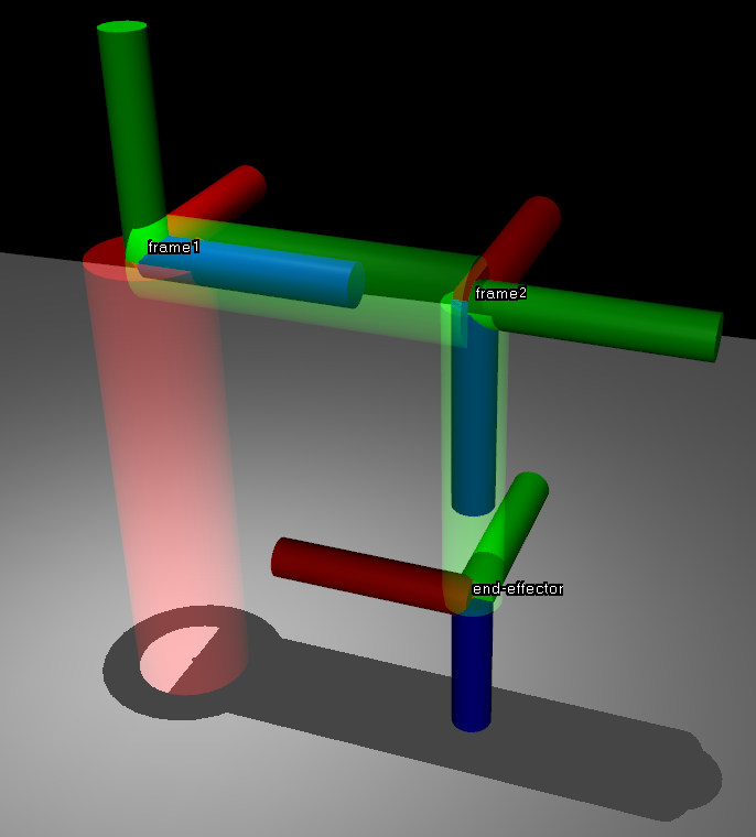
In this section we will be showing that the forward and inverse kinematic equations derived in question 1 and 2 are correct by simulating the pendulum in MuJoCo and extracting from the end effector frame and frame 2.
Our MuJoCo model looks like this:
Methodology and Results
Verifying Question 1 Parts A, B, and C
In question 1, we found these pose matrixes with the given angles $\theta_1 = \pi/3$ and $\theta_2=-3\pi/7$:
$$ ^{0}T_{c} = \left[\begin{matrix}-0.5 & -0.193 & 0.844 & 1.075\\-0.866 & 0.111 & -0.487 & 0.303\\0.0 & -0.975 & -0.223 & 1.022\\0.0 & 0.0 & 0.0 & 1.0\end{matrix}\right] $$
$$ ^{0}T_{2} = \left[\begin{matrix}-0.193 & 0.5 & 0.844 & 0.4\\0.111 & 0.866 & -0.487 & 0.693\\-0.975 & 0.0 & -0.223 & 1.2\\0.0 & 0.0 & 0.0 & 1.0\end{matrix}\right] $$
To verify that these are correct, we will plug in these $\theta$ values and see if we get the same pose back. Our simulated results are:
$$ ^{0}T_{c} = \left[\begin{matrix}-0.5 & -0.193 & 0.844 & 1.075\\-0.866 & 0.111 & -0.487 & 0.303\\0.0 & -0.975 & -0.223 & 1.022\\0.0 & 0.0 & 0.0 & 1.0\end{matrix}\right] $$
$$ ^{0}T_{2} = \left[\begin{matrix}-0.193 & 0.5 & 0.844 & 0.4\\0.111 & 0.866 & -0.487 & 0.693\\-0.975 & 0.0 & -0.223 & 1.2\\0.0 & 0.0 & 0.0 & 1.0\end{matrix}\right] $$
Which is exactly the same as our calculated result.
It should be noted that these numbers are rounded, and there are minor discrepancies that are negligible and explainable through numerical computation methods in the simulation.
This verifies question 1 parts a, b, and c since the axis-angle and quaternion representations of the orientation are obviously be the same because the orientations are the same.
Verifying Question 1 Part D
In part d, we found 2 sets of solutions that result in the desired orientation of the z-axis of frame c.
Desired orientation of the z-axis: $$ k = -\frac{1}{2} x_0 + \frac{1}{2} y_0 - \frac{\sqrt{2}}{2} z_0. $$
Solution 1: $$ (\theta_1, \theta_2) = (-0.7854, 5.4978) $$
Resulted in this pose: $$ \begin{bmatrix} 0.7071 & 0.5 & -0.5 & -0.9657 \\ 0.7071 & -0.5 & 0.5 & -0.1657 \\ 0 & -0.7071 & -0.7071 & 0.6343 \\ 0 & 0 & 0 & 1 \end{bmatrix} $$
Solution 2: $$ (\theta_1, \theta_2) = (2.356, 0.7854) $$
Resulted in this pose: $$ \begin{bmatrix} -0.7071 & -0.5 & -0.5 & 0.1657 \\ -0.7071 & 0.5 & 0.5 & 0.9657 \\ 0 & 0.7071 & -0.7071 & 0.6343 \\ 0 & 0 & 0 & 1 \end{bmatrix} $$
If we plug these new $\theta$ values into the simulation, we should see the same pose matrixes come out of it.
Plugging $\theta_1$ and $\theta_2$ in result in:
Pose 1, corresponding to solution 1:
$$ \left[\begin{matrix}0.7071 & 0.5 & -0.5 & -0.9657\\0.7071 & -0.5 & 0.5 & -0.1657\\0.0 & -0.7071 & -0.7071 & 0.6343\\0.0 & 0.0 & 0.0 & 1.0\end{matrix}\right] $$
Pose 2, corresponding to solution 2:
$$ \left[\begin{matrix}-0.7071 & -0.5 & -0.5 & 0.1657\\-0.7071 & 0.5 & 0.5 & 0.9657\\0.0 & 0.7071 & -0.7071 & 0.6343\\0.0 & 0.0 & 0.0 & 1.0\end{matrix}\right] $$
As can be seen, the calculated and simulated pose matrixes are the same, verifying our calculations.
Verifying Question 1 Part E
In part e, we found 2 sets of solutions that result in the desired position of frame c.
Desired position of frame c: $$ p = 1.075x_0 + 0.303y_0 + 1.022z_0. $$
Solution 1: $$ (\theta_1, \theta_2) = (1.0727, 1.3464) $$
Resulted in this pose: $$ \begin{bmatrix} -0.8785 & 0.1063 & 0.4658 & 1.0754 \\ 0.4777 & 0.1955 & 0.8565 & 0.303 \\ 0 & 0.9749 & -0.2225 & 1.022 \\ 0 & 0 & 0 & 1 \end{bmatrix} $$
Solution 2: $$ (\theta_1, \theta_2) = (2.6181, 4.9368) $$
Resulted in this pose: $$ \begin{bmatrix} -0.4999 & -0.1927 & 0.8444 & 1.0754 \\ -0.8661 & 0.1112 & -0.4873 & 0.303 \\ 0 & -0.9749 & -0.2225 & 1.022 \\ 0 & 0 & 0 & 1 \end{bmatrix} $$
Pose 1, corresponding to solution 1:
$$ \left[\begin{matrix}-0.8785 & 0.1063 & 0.4658 & 1.0754\\0.4777 & 0.1955 & 0.8565 & 0.303\\0.0 & 0.9749 & -0.2225 & 1.022\\0.0 & 0.0 & 0.0 & 1.0\end{matrix}\right] $$
Pose 2, corresponding to solution 2:
$$ \left[\begin{matrix}-0.4999 & -0.1927 & 0.8444 & 1.0754\\-0.8661 & 0.1112 & -0.4873 & 0.303\\0.0 & -0.9749 & -0.2225 & 1.022\\0.0 & 0.0 & 0.0 & 1.0\end{matrix}\right] $$
As can be seen, the calculated and simulated pose matrixes are the same, verifying our calculations.
Verifying Question 2 Part A and B
We were given some joint angles and velocities and asked to produce body and spacial twists for frame c and frame 2.
The joint angles $\theta$ were given by
$$ \theta = \begin{bmatrix} \theta_1 \\ \theta_2 \end{bmatrix} = \begin{bmatrix} 5\pi/6 \\ -3\pi/7 \end{bmatrix} $$
The angular rates of change were also given:
$$ \dot{{\theta}} = \begin{bmatrix} 1 & 2 \end{bmatrix}^{\top} $$
The resulting twists were calculated:
$$ {}^0V_c^0 = \left[\begin{matrix}v\\\omega\end{matrix}\right] = \left[\begin{matrix}-2.079\\1.2\\0\\1.0\\1.732\\1.0\end{matrix}\right] , {}^cV_c^0 = \left[\begin{matrix}v\\\omega\end{matrix}\right] = \left[\begin{matrix}-0.780\\1.778\\-0.78\\-2.0\\-0.975\\-0.223\end{matrix}\right] ,\\ \ \\ {}^0V_2^0 = \left[\begin{matrix}v\\\omega\end{matrix}\right] = \left[\begin{matrix}-2.079\\1.2\\0\\1.0\\1.732\\1.0\end{matrix}\right] , {}^2V_2^0 = \left[\begin{matrix}v\\\omega\end{matrix}\right] = \left[\begin{matrix}0.178\\0\\-0.780\\-0.975\\2.0\\-0.223\end{matrix}\right] $$
We can verify this in MuJoCo by plugging in the joint angles and velocities and seeing if the resulting simulated twist matches with our calculated twist.
Plugging these values in we get:
$$ {}^0V_c^0 = \left[\begin{matrix}-2.078\\1.2\\0.0\\1.0\\1.732\\1.0\end{matrix}\right], \ {}^cV_c^0 = \left[\begin{matrix}-0.78\\1.778\\-0.78\\-2.0\\-0.975\\-0.223\end{matrix}\right] \\ \ \\ {}^0V_2^0 = \left[\begin{matrix}-2.078\\1.2\\0.0\\1.0\\1.732\\1.0\end{matrix}\right] , {}^2V_2^0 = \left[\begin{matrix}0.178\\0.0\\-0.78\\-0.975\\2.0\\-0.223\end{matrix}\right] $$ It should be noted that the spatial twist found in both frames was derived by doing an ad-joint transformation on the body twist found via mujoco simulation.
${}^AV_B = \text{Ad}_{^{A}T_B} {}^BV_B$
As can be seen, the calculated and simulated twist matrixes are the same, verifying our calculations. There is a slight difference in the x component of the linear velocities in the spatial of 0.001, however this difference can be attributed to the RK4 integrator.
Verifying Question 2 Part C and D
We were given the following twists and asked to find the joint rates.
Given body twist: $$ {}^cV_c^0 = (\mathbf{v}_c, \boldsymbol{\omega}_c) = \begin{bmatrix} 0.39 & 0.871 & 0.39 & -1.2 & 0.487 & 0.111 \end{bmatrix}^{\top} $$ Given spatial twist: $$ {}^0V_c^0 = (\mathbf{v}_c, \boldsymbol{\omega}_c) = \begin{bmatrix} -1.247 & 0.72 & 0 & 0.6 & 1.039 & -0.5 \end{bmatrix}^{\top} $$
The joint rates we found for each twist were the same: $$ \dot{\theta}_1 = -0.5 \text{ rad/s}, \quad \dot{\theta}_2 = 1.2 \text{ rad/s} $$
We can verify this in MuJoCo by plugging in the joint rates we found and seeing if the resulting simulated twist matches with the given twist.
Plugging in these joint rates into the simulation:
$${}^cV_c^0 = \left[\begin{matrix}0.39\\0.871\\0.39\\-1.2\\0.487\\0.111\end{matrix}\right]$$
$${}^0V_c^0 = \left[\begin{matrix}-1.247\\0.72\\0.0\\0.6\\1.039\\-0.5\end{matrix}\right]$$
As can be seen, the calculated and simulated twist matrixes are the same, verifying our calculations.
Simulation of Sgn Function Actuation (Question 4)
Question 4 is a bit different from the rest of the questions as it mostly involves coding. In question 4 the pendulum starts at the home position and is driven by an actuator at frame one which applies a torque given by: $$\tau = -15 \operatorname{sgn} \dot{\theta}_2$$
The code sets up the model and then steps through the simulation at a rate of 2ms per step using a RK4 integrator. The simulation loop is shown below:
# Start the simulation loop
time_simulated = 0
time_to_simulate = 15#s
show_in_real_time = False
with mujoco.viewer.launch_passive(model, data) as viewer:
    steps = 0
    while viewer.is_running():
        # Set current control input
        data.ctrl[actuator_id] = -15 * np.sign(data.qvel[1].copy())

        # Step simulation
        mujoco.mj_step(model, data)

        if show_in_real_time:
            #Update viewer
            viewer.sync()
            #Sleep so you can watch the simulation in real time.
            time.sleep(0.002)
        time_simulated += .002
        steps += 1
        #Now we are ready to record data for this step.
        heights.append(data.xpos[end_effector_body_id][2])
        times.append(time_simulated)
        body_lin_vels_endeffector.append(data.sensordata[:3].copy())
        R0c = data.xmat[frame1_body_id].reshape(3,3)
        spatial_ang_vels_endeffector.append(np.array(R0c) @ np.array(data.sensordata[3:6].copy()))
        spatial_ang_vels_frame_1.append(np.array(R0c) @ np.array(data.sensordata[6:9].copy()))

        # Stop the simulation after is has simulated the desired time.
        if time_simulated > time_to_simulate:
            break

print("Done Simulating")
Then the code proceeds to plot the data as requested, the plots are shown below:
Heights graph
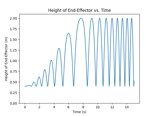
From this graph we see that the heights gradually increased, and stayed between 0.4m and 2m. This is because the end-effector can only be in that height range due to the geometry of the pendulum.
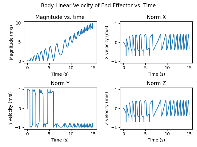
The second graph shows that for the first 6 seconds the magnitude of the velocity oscillates between an ever increasing value and 2. This is the result of the pendulum swinging back and forth to greater and greater heights. Then after 6 seconds it is able to complete a full rotation and the velocity no longer stops at zero. As the pendulum continues to swing it goes faster and faster which explains why the oscillations get smaller and smaller. Finally I conjecture that the linear rate of the increase of the velocity peaks is due to a sort of constant rate of energy transfer into the system.
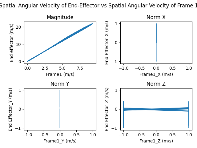
The last graph is also rather interesting. It graphs the end effector angular velocity versus the angular velocity of frame 1. The straight line in the magnitude graph indicates that the velocities of the two joints are proportional. This makes sense because the end-effector is has less inertia than the other links so it is reasonable for its angular velocity to be relatively faster. The vertical lines on the X and Y direction are a result of the fact that joint 1 can only rotate about the Z axis, which necessitates that its angular velocity be 0 in the X and Y directions.
Images
Here is an image of the simulation